


Machine learning algorithms are the backbone of intelligent systems, allowing them to identify patterns, make predictions, and improve over time. Machine learning algorithms are mathematical models that enable systems to learn from data and automatically improve.
Types of ML algorithms (supervised, unsupervised, and reinforcement) are used in a wide range of industries, from healthcare to finance. Our machine learning development services are designed for enterprises, startups, and product teams seeking more intelligent automation. With the help of top 10 algorithms, you will achieve accurate predictions, reduced operational costs, and scalable AI solutions.
By 2026, the machine learning algorithm market will exceed $100 billion. Random forests provide a prediction bias of less than 3%; SVMs deliver accuracy on high-dimensional data, improving ROI in finance, retail, and healthcare.
This article will examine the most frequently used algorithms.
Use the best machine learning algorithms today as the top 10 are the foundation of any profitable AI strategy.
1. Linear Regression
Simple and Widely Used Algorithm for Predicting Continuous Target Variables. Linear regression(LR) is a fundamental statistical method used extensively in data science and machine learning for predicting a continuous target variable based on one or more input features. Its simplicity and interpretability make it a popular choice for both beginners and experienced practitioners.
What is Linear Regression?
LR seeks to represent the relationship between a dependent variable (target) and one or more independent variables (features) by fitting a linear equation to the observed data. The general form is:
\( y = w_0+ w_1∙ x_1 + w_2∙ x_2 +…+ w_n∙ x_n + ε \)
Where:
y is the dependent variable.
\( x_1, x_2, x_n \)are the independent variables.
\( w_0 \)is the intercept.
\( w_1, w_2, w_n \)are the coefficients.
\( ε \)is the error term.dw
Types of LR:
Simple LR: Involves a single independent variable. The relationship is modeled as a straight line:
\( y = w_0+ w_1∙ x_1 + ε \)
Multiple LR:
\( y = w_0+ w_1∙ x_1 + w_2∙ x_2 +…+ w_n∙ x_n + ε \)
On each point there are two values – actual and the predicted value of the model. LR calculates the squared discrepancies between them. This is achieved using a method called Ordinary Least Squares (OLS).
2. Logistic Regression
Logistic regression is a fundamental statistical method used for binary classification tasks. It forecasts the likelihood of a binary result, which can be 0 or 1, true or false. This technique is widely used in various fields, including medicine, finance, and social sciences, due to its simplicity and effectiveness.
Understanding Logistic Regression
In contrast to LR, which forecasts a continuous outcome, logistic regression is employed when the dependent variable is categorical. The logistic function, or sigmoid function, is fundamental to logistic regression. It maps any real-valued number into a value between 0 and 1, making it suitable for probability estimation.
The logistic function is defined as:
sigma(z) = 1/(1 + e^(-z))
where ( z ) is the linear combination of input features.
Training a logistic regression model involves finding the best-fitting parameters (weights) that minimize the difference between the predicted probabilities and the actual binary outcomes.This is usually accomplished through a technique known as maximum likelihood estimation (MLE). Logistic regression remains a powerful and widely-used tool for binary classification tasks. Its ability to provide probability estimates makes it particularly valuable in fields where decision-making is based on risk assessment and prediction.
3. Support Vector Machine (SVM)
What is a support vector machine? The method is related to binary classifiers (when there are only two classes). The idea of SVM is simple at its core: it looks for how to draw two lines between categories to create the largest gap.
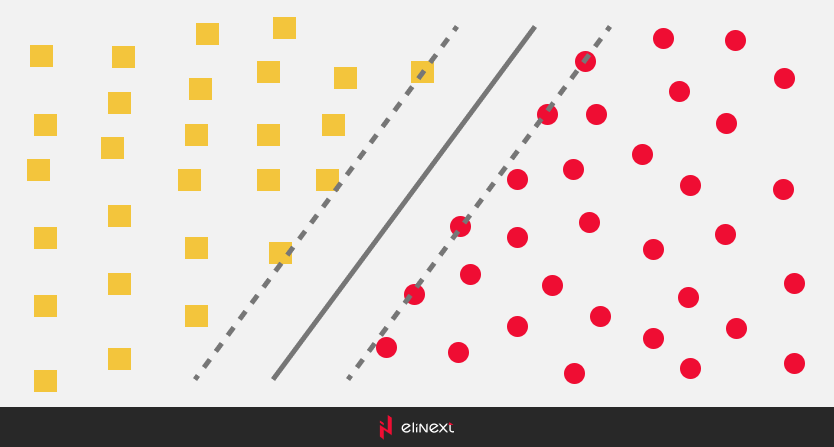
In more scientific terms, we can say this: a support vector machine (SVM) is a machine learning algorithm that is used for classification and regression. It is based on the idea that data points can be divided into two groups using a hyperplane that passes through these points.
In order to build this hyperplane, the support vector machine uses so-called support vectors, which are data points lying on the border between the groups. These support vectors are used to determine the direction and distance from the hyperplane to each data point.
In this way, the support vector machine allows you to determine which group the data points belong to and use this data to create a model that can be used to predict new data.
What you need to know to understand the SVM:
The mathematical foundations of support vector machines. SVM is based on a linear model that defines a hyperplane that separates the data into two categories.
Choosing a kernel function. Choosing a kernel function is a key factor when using SVM. The kernel function allows SVM to work with nonlinear functions, which can improve its performance on some problems.
Optimizing hyperparameters. SVM has several hyperparameters that need to be tuned to achieve the best results. These parameters include the regularization coefficient, error penalty, kernel function, and so on.
Fitting the model. After tuning the hyperparameters, you need to fit the model on the training data. This involves calculating the hyperplane coefficients and optimizing the objective function.
Evaluating the quality of the model. After fitting the model, you need to evaluate its quality on the test data.
4. Decision Tree
Decision trees work by splitting the data into branches based on feature values, making it easy to understand and visualize. Decision trees are widely used in various fields, including finance, healthcare, and marketing, due to their simplicity and effectiveness.
A decision tree consists of nodes and branches. Each internal node represents a decision based on a feature, each branch represents the outcome of that decision, and each leaf node represents a final prediction or outcome. The process of building a decision tree involves selecting the best feature to split the data at each node, which is typically done using criteria like Gini impurity or information gain.
Key Concepts:
- Root Node: The topmost node in a decision tree, representing the entire dataset.
Internal Nodes: Nodes that represent decisions based on feature values.
- Leaf Nodes: Terminal nodes that represent the final prediction or outcome.
- Splitting: The process of dividing a node into two or more sub-nodes based on a feature.
- Pruning: The process of removing parts of the tree to prevent overfitting and improve generalization.
The procedure for constructing a decision tree includes these steps:
- Select the Best Feature: Choose the feature that best splits the data based on a chosen criterion (e.g., Gini impurity, information gain).
- Split the Data: Divide the dataset into subsets based on the selected feature.
- Repeat: Recursively apply the process to each subset until a stopping condition is met (e.g., maximum depth, minimum samples per leaf).
5. Random Forest
This approach utilizes collective intelligence by combining the forecasts of multiple decision trees, resulting in a more precise and reliable model with machine learning algorithms. Random Forest is composed of numerous individual decision trees that function together as an ensemble. Each tree in the forest is built from a random subset of the training data and a random subset of features. The final prediction is made by averaging the predictions of all the trees (for regression) or by taking a majority vote (for classification).
Key Concepts:
- Bootstrap Aggregation (Bagging): Random Forest uses bagging to create multiple subsets of the original dataset by sampling with replacement. Each subset is used to train a different decision tree.
- Random Feature Selection: At each split in the decision tree, a random subset of features is considered, which helps in reducing correlation among the trees and improving model diversity.
- Ensemble Prediction: The predictions from all the trees are combined to produce the final output, which helps in reducing variance and improving accuracy.
The process of building a Random Forest:
- Create Bootstrapped Datasets: Generate multiple subsets of the training data by sampling with replacement.
- Train Decision Trees: Build a decision tree for each subset using a random subset of features at each split.
- Aggregate Predictions: Combine the predictions from all the trees to make the final prediction.
6. Naive Bayes Classifier
This algorithm is particularly effective for text classification tasks, such as spam detection, sentiment analysis, and document categorization. Despite its simplicity, Naive Bayes often performs surprisingly well and is a popular choice for many real-world applications. Naive Bayes classifiers assume that the features are conditionally independent given the class label, which is a strong assumption and often not true in practice. However, this “naive” assumption simplifies the computation and works well in many scenarios.
Naive Bayes is expressed as:
\( P(C|X) =(P(X|C) ∙ P(C))/(P(X)) \)
Where:
P(C|X) is the posterior probability of class ( C ) given the features ( X ).
P(X|C)) is the likelihood of features ( X ) given class ( C ).
P(C) is probability of class ( C ).
P(X) is probability of features ( X ).
Types of Naive Bayes Classifiers
- Multinomial Naive Bayes: Suitable for discrete data, commonly used for text classification where features represent word frequencies.
- Bernoulli Naive Bayes: Used for binary/boolean features, such as the presence or absence of a word in a document.
- Gaussian Naive Bayes: Assumes that the features follow a normal distribution, used for continuous data.
The Naive Bayes classifier is a robust and efficient tool for text classification tasks. Its probabilistic nature and simplicity make it a valuable asset in the machine learning toolkit, especially for applications involving large datasets and high-dimensional feature spaces.
7. K-Nearest Neighbors (KNN)
K-Nearest Neighbors (KNN) is a non-parametric, instance-based learning algorithm used for classification and regression tasks. It categorizes data points by identifying the predominant class among their closest neighbors within the feature space. Despite its simplicity, KNN is highly effective and widely used in various applications, including pattern recognition, data mining, and intrusion detection.
Understanding KNN:
KNN operates on the principle that similar data points are likely to be close to each other in the feature space. The algorithm determines the class of a new data point by examining the ‘k’ nearest neighbors and assigning it the most frequent class among them. The value of ‘k’ is a crucial parameter that determines the number of neighbors considered.
Algorithm Steps:
- Choose the Number of Neighbors (k): Select the number of nearest neighbors to consider.
- Calculate Distance: Compute the distance(Manhattan, Euclidean, Minkowski) between the new data point and all other points in the dataset.
- Identify Nearest Neighbors: Select the ‘k’ data points with the smallest distances to the new point.
- Classify: Assign the class label that is most frequent among the ‘k’ nearest neighbors.
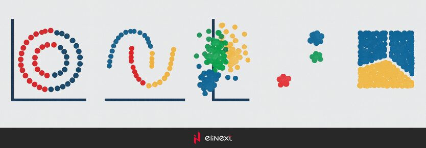
8. K-Means Clustering
K-Means Clustering is a popular unsupervised learning algorithm used to partition data into (k) clusters based on feature similarity. It is widely used in various fields such as market segmentation, image compression, and pattern recognition. The algorithm aims to minimize the variance within each cluster, making it a powerful tool for discovering underlying patterns in data.
The K-Means algorithm works by iteratively assigning data points to clusters and updating the cluster centroids until convergence. The goal is to partition the data into ( k ) clusters where each data point belongs to the cluster with the nearest mean (centroid).
Algorithm Steps:
- Initialize Centroids: Randomly select ( k ) data points as initial cluster centroids.
- Assign Clusters: Assign each data point to the nearest centroid based on a distance metric (commonly Euclidean distance).
- Update Centroids: Calculate the new centroids by taking the mean of all data points assigned to each cluster.
- Repeat: Repeat the assignment and update steps until the centroids no longer change significantly or a maximum number of iterations is reached.
K-Means Clustering’s simplicity and efficiency make it a popular choice for various applications, from market segmentation to image compression. However, careful consideration of the number of clusters and initialization methods is essential to achieve optimal results.
9. Clustering with DBSCAN
DBSCAN (Density-Based Spatial Clustering of Applications with Noise) is a powerful unsupervised learning algorithm used for clustering tasks. Unlike traditional clustering methods like K-Means, DBSCAN can identify clusters of arbitrary shape and is particularly effective at handling noise and outliers. It is widely used in fields such as geospatial analysis, image processing, and anomaly detection.
DBSCAN groups together points that are closely packed, marking points that are far away from others as outliers. The algorithm relies on two key parameters: epsilon (ε), which defines the radius of a neighborhood around a point, and minPts, the minimum number of points required to form a dense region (cluster).
Algorithm Steps:
- Select a Point: Start with an arbitrary point in the dataset.
- Neighborhood Check: Find all points within the ε radius of the selected point.
- Core Point Identification: If the number of points in the neighborhood is greater than or equal to minPts, mark the point as a core point and form a cluster.
- Expand Cluster: Recursively add all density-reachable points (points within ε distance of any point in the cluster) to the cluster.
- Repeat: Continue the process for all points in the dataset.

Clustering using the steps of the DBSCAN algorithm
10. Principal Component Analysis (PCA)
Principal Component Analysis (PCA) is a popular method in statistics for reducing the number of dimensions in a dataset. It reduces high-dimensional data to a lower-dimensional format, maintaining as much variability as possible. PCA is particularly useful in fields like data visualization, image processing, and exploratory data analysis, where reducing the number of variables can simplify models and highlight important patterns.
Understanding PCA:
PCA operates by finding the directions (principal components) that maximize the variance within the data. These principal components are orthogonal to each other, ensuring that they capture distinct patterns in the data. The first principal component explains the most variance, with the second capturing the next highest amount, and so on.
Algorithm Steps:
- Standardize the Data: Ensure that each feature has a mean of zero and a standard deviation of one.
- Compute the Covariance Matrix: Calculate the covariance matrix to understand how the features vary with respect to each other.
- Calculate Eigenvalues and Eigenvectors: Determine the eigenvalues and eigenvectors of the covariance matrix. The eigenvectors represent the principal components, and the eigenvalues indicate the amount of variance captured by each component.
- Sort and Select Principal Components: Sort the eigenvalues in descending order and select the top ( k ) eigenvectors corresponding to the largest eigenvalues.
- Transform the Data: Project the original data onto the selected principal components to obtain the reduced-dimensional representation.
By transforming high-dimensional data into a lower-dimensional form, PCA helps in uncovering important patterns and simplifying complex datasets.
In Industry 4.0, most enterprises collect massive amounts of data but lack the structure to process it. The wrong types of machine learning algorithms take months to develop. At Elinext, our AI software development services match each algorithm to a specific business problem, from fraud detection with SVMs to demand forecasting with random forests.” The result: faster deployment, reduced development costs, and models that scale with your data.
Senior Machine Learning Engineer, Elinext
Conclusion
The top 10 machine learning algorithms remain the foundation of modern AI implementation. In 2025, the global machine learning market reached $74.95 billion, demonstrating a CAGR of 30.4%. Machine learning algorithms, from linear regression to neural networks, are now used in healthcare, finance, and manufacturing. McKinsey reports that data-driven organizations are 19 times more likely to achieve profitability. For example, a retailer using the Random Forest algorithm reduced its forecasting error to less than 3%. Investing in the right machine learning algorithms is now the most obvious path to competitive advantage.
Machine Learning Algorithms: Terms Explained
-
Machine Learning
Machine learning is a branch of artificial intelligence in which systems learn patterns in data without explicit programming. It underlies product recommendations, fraud detection, and medical diagnostics and automatically improves accuracy as new data is received.
-
Supervised Learning
Supervised learning is a type of machine learning in which a model is trained on labeled input-output pairs. It is used for classification and regression problems. For example, predicting customer churn or diagnosing diseases based on historical patient records.
-
Unsupervised Learning
Unsupervised learning finds hidden patterns in unlabeled data. Algorithms such as K-means clustering group customers by behavior without predefined categories, helping businesses identify market segments and reduce data complexity independently.
-
Linear Regression
Linear regression models the relationship between a dependent variable and one or more predictors using a straight line. It is widely used for sales forecasting, price estimation, and risk assessment due to its simplicity and interpretability.
-
Decision Tree
A decision tree divides data into branches based on feature values to achieve a prediction. It is favored in regulated industries such as banking and healthcare due to its transparency. Each decision path is human-readable and easily verifiable.
-
Random Forest
A random forest is an ensemble of multiple decision trees that vote on the final output. It reduces overfitting and copes well with noisy data. In retail demand forecasting, it achieved forecast biases of -1% to +3%
-
Support Vector Machine
A support vector machine finds the optimal boundary separating classes in a high-dimensional space. It is excellent for text classification, image recognition, and bioinformatics problems where the feature dimensionality significantly exceeds the number of samples.
-
Neural Network
A neural network is a multi-layered system of interconnected nodes modeled after the human brain. It underpins deep learning applications such as speech recognition, autonomous driving, and medical imaging.
FAQ
Which machine learning algorithm is best for beginners?
Types of machine learning algorithms vary in complexity. Linear regression is best for beginners: simple, interpretable, and ideal for predicting house prices.
Why is Random Forest widely used?
Machine learning algorithms vary in robustness. The Random Forest algorithm combines multiple trees to filter out errors and handle missing data proven to have a bias of less than 3% in retail.
When should you use a Support Vector Machine?
Different types of ML algorithms are suited to different types of data. Use a support vector machine for small, high-dimensional datasets. For example, classifying cancer by gene expression.
Which algorithm works best for classification problems?
Machine learning algorithms handle classification differently. Random Forest excels on structured data; neural networks dominate image and text classification tasks.
Which machine learning algorithm is best for large datasets?
Types of machine learning algorithms scale differently. Neural networks and gradient boosting excel at handling large datasets and are ideal for processing millions of daily transactions or IoT streams.
Are all machine learning algorithms supervised?
Not all machine learning algorithms are supervised. These include supervised, unsupervised, and reinforcement learning algorithms and the K-means algorithm clusters unlabeled data.
How do you choose the right machine learning algorithm?
Machine learning algorithms are chosen by problem type and data size. Define classification vs. regression, check volume, then test 2–3 candidates on a validation set.
